The use of this site and the content contained therein is governed by the Terms of Use. When you use this site you acknowledge that you have read the Terms of Use and that you accept and will be bound by the terms hereof and such terms as may be modified from time to time.
All text, graphics, audio, design and other works on the site are the copyrighted works of nasscom unless otherwise indicated. All rights reserved.
Content on the site is for personal use only and may be downloaded provided the material is kept intact and there is no violation of the copyrights, trademarks, and other proprietary rights. Any alteration of the material or use of the material contained in the site for any other purpose is a violation of the copyright of nasscom and / or its affiliates or associates or of its third-party information providers. This material cannot be copied, reproduced, republished, uploaded, posted, transmitted or distributed in any way for non-personal use without obtaining the prior permission from nasscom.
The nasscom Members login is for the reference of only registered nasscom Member Companies.
nasscom reserves the right to modify the terms of use of any service without any liability. nasscom reserves the right to take all measures necessary to prevent access to any service or termination of service if the terms of use are not complied with or are contravened or there is any violation of copyright, trademark or other proprietary right.
From time to time nasscom may supplement these terms of use with additional terms pertaining to specific content (additional terms). Such additional terms are hereby incorporated by reference into these Terms of Use.
Disclaimer
The Company information provided on the nasscom web site is as per data collected by companies. nasscom is not liable on the authenticity of such data.
nasscom has exercised due diligence in checking the correctness and authenticity of the information contained in the site, but nasscom or any of its affiliates or associates or employees shall not be in any way responsible for any loss or damage that may arise to any person from any inadvertent error in the information contained in this site. The information from or through this site is provided "as is" and all warranties express or implied of any kind, regarding any matter pertaining to any service or channel, including without limitation the implied warranties of merchantability, fitness for a particular purpose, and non-infringement are disclaimed. nasscom and its affiliates and associates shall not be liable, at any time, for any failure of performance, error, omission, interruption, deletion, defect, delay in operation or transmission, computer virus, communications line failure, theft or destruction or unauthorised access to, alteration of, or use of information contained on the site. No representations, warranties or guarantees whatsoever are made as to the accuracy, adequacy, reliability, completeness, suitability or applicability of the information to a particular situation.
nasscom or its affiliates or associates or its employees do not provide any judgments or warranty in respect of the authenticity or correctness of the content of other services or sites to which links are provided. A link to another service or site is not an endorsement of any products or services on such site or the site.
The content provided is for information purposes alone and does not substitute for specific advice whether investment, legal, taxation or otherwise. nasscom disclaims all liability for damages caused by use of content on the site.
All responsibility and liability for any damages caused by downloading of any data is disclaimed.
nasscom reserves the right to modify, suspend / cancel, or discontinue any or all sections, or service at any time without notice.
For any grievances under the Information Technology Act 2000, please get in touch with Grievance Officer, Mr. Anirban Mandal at data-query@nasscom.in.
Functional safety is a vital discipline in engineering, focusing on ensuring system safety in areas impacting human safety or the environment. It aims to prevent or minimize the consequences of system failures, faults, or errors leading to hazardous situations.
The complexity of modern systems in critical industries such as aerospace, automotive, and medical devices necessitate rigorous functional safety verification. This verification process ensures correct implementation of safety measures and addresses potential hazards before deployment. It involves comprehensive testing, analysis, and simulation to validate system behavior under normal and abnormal conditions.
Examples highlight the significance of functional safety across industries. For instance, in automotive applications, airbag systems must reliably deploy to protect occupants during accidents. Similarly, medical devices like pacemakers require continuous and reliable operation to avoid life-threatening consequences for patients.
In automotive engineering, functional safety is paramount due to the interconnected nature of vehicle systems. Electronic control units (ECUs) manage critical functions like braking and steering, necessitating seamless system interaction for safety and performance. Compliance with stringent safety standards, such as ISO 26262, is not only a regulatory requirement but also crucial for protecting lives on the road.
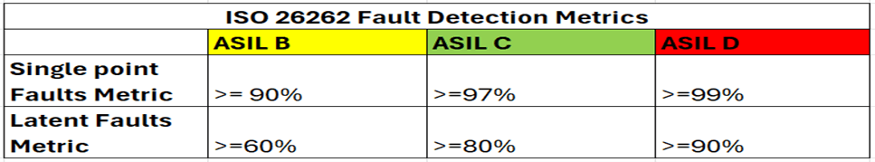
The ISO26262 standard provides a guideline to assess severity of all situations and provides a safety rating system called Automotive Safety Integrity Level (ASIL).
Fig 2: ISO 26262 Fault Detection Metrics
Focusing on the ASIL-B standard, the system should be capable of identifying 90% of single point faults occurring in the design using all the SMs (safety mechanism) defined for that design.
Fault injection
Fault injection is a technique used in functional safety verification to assess how a system responds to various faults or errors intentionally introduced into its operation. By simulating faults, engineers can evaluate the system’s robustness and its ability to detect, diagnose, and recover from potential failures.
ISO26262 function safety standard verification requires extensive fault injection campaigns and complex manual analysis.
Faults can be broadly classified into Permanent and Transient. A permanent fault is a type of fault that persists until it is actively corrected or repaired. It occurs due to inherent functional errors in the design, component degradation, manufacturing defect, physical damage, electromagnetic interference, etc. A transient fault is a temporary deviation from normal system behavior that occurs due to external factors or temporary conditions. Unlike permanent faults that persist until corrected, transient faults typically resolve on their own once the influencing factor diminishes. It occurred due to voltage spikes, electrostatic discharge, environment factors, radiation or cosmic rays, interference from nearby equipments, etc.
Permanent fault can be simulated by forcing 0 or 1 on the node, classified as stuck at 0 and stuck at 1 fault. Gate level netlist is used for fault injection of permanent fault model. In transient fault, the signal is inverted, and the modified value remains for a small time. This is classified into two types-
Single event upset (SEU): Faulty value remains until new value assigned
Single event transient (SET): Hold the value for a specific period of time
The Fault Campaign Manager (FCM) oversees the entirety of the fault injection campaign, managing every step from planning to execution. It relies on critical engines such as the Xcelium Fault Simulator (XFS) and the Jasper Functional Safety Verification App (FSV) to create a robust and thorough functional safety solution. These tools work together seamlessly within the FCM framework, allowing for comprehensive fault injection testing, data analysis, and reporting.
The FCM ensures that fault scenarios are configured accurately, simulations are run effectively, and results are analysed comprehensively to assess system resilience, fault tolerance, and safety mechanisms. By integrating these core engines, the FCM streamlines the end-to-end flow of functional safety verification, enabling engineers to validate safety requirements and enhance system reliability efficiently. The steps for FCM flow are given below:
Fig 4: Fault Injection Campaign
PREP: Create campaign directory structure
O_EXEC, O_RANK: Execute all test cases from users list and rank the test cases for fault injection (FI) (based on toggle coverage percentage contribution by each test cases).
G_ELAB: Elaborate the design with fault information, create xcelium snapshot and fault database
FST: Fault space reduction using testability analysis and cone of influence (COI)
FSV_TC: Fault pruning with constant analysis
F_EXEC, F_EXEC_C: Simulate each fault with selected rank test cases using concurrent and serial engines
F_RANK: Generate final report with fault details
Challenges and Solutions
There are lot of challenges while using FCM flow for bigger IPs (large fault lists). Challenges and effective solutions are provided below:
Addressing runtime issues
Optimizing fault list
Test case prioritization
Utilizing engineering judgment
Understanding tools limitation
Selection of window of opportunity
Addressing runtime issues
Runtime issues can be classified into two:
Huge runtime for complex designs (large fault list)
Handling non simulatable (NS) fault
Huge runtime for complex designs
Designs containing fewer than 50,000 faults can complete the campaign relatively quickly.
However, designs exceeding 50,000 faults, such as hardware accelerator designs with over 1 million faults, will require more time. It is possible to reduce runtime by configuring parameters appropriately.
Grouping is a crucial parameter in fault injection campaigns. Consider a scenario with 5000 faults and 10 test cases, resulting in 50000 fault simulations (5000 faults * 10 test cases). Executing such a large number of simulations can significantly prolong the campaign duration. Grouping faults offers an effective solution to this challenge.
For instance, if we group 1000 faults per simulation, only 5 simulations will be necessary for each test case, reducing the total simulations to 50 for the entire fault injection campaign. This grouping strategy significantly decreases the campaign’s runtime. Moreover, if there are sufficient licenses, all 50 simulations can run concurrently, further reducing the overall runtime.
However, it is essential to note a potential drawback of grouping: simulating 1000 faults in a single simulation may take longer than simulating 1 fault per simulation. This trade-off between the number of faults per simulation and simulation runtime should be carefully considered based on the specific requirements and constraints of the fault injection testing process.
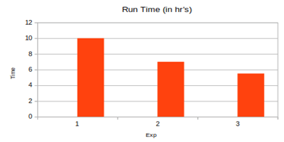
We need to determine the optimal value for fault grouping based on the number of faults, test cases, and available fault simulator licenses. Conducting experiments to find the most effective grouping value is crucial. Below are the details of the experiments conducted and the findings regarding the best value for fault grouping.
A limitation exists with the concurrent engine regarding faults labelled as non-simulatable, particularly when these faults propagate through RTL constructs (e.g., behavioural memory code). These non-simulatable (NS) faults are executed by the serial engine, which can extend the runtime.
To mitigate this issue and improve runtime, reducing the number of NS faults is essential. One approach is to define a fault boundary, which delineates the extent of fault propagation. For example, when analysing a specific IP (Intellectual Property), it is beneficial to align the fault boundary with the IPs boundaries or the hierarchy where checker strobes and functional strobes are located. This strategy effectively reduces non-simulatable faults, thereby decreasing the need for serial runs and optimizing overall runtime.
Optimizing fault list
After the simulation phase, numerous undangerous undetected (UU) faults may remain, which are not observed in functional and checker strobes. Generally, faults become UU due to two reasons: either there are no test cases to exercise the fault path, or the fault itself is considered safe. To streamline fault simulation and reduce total faults, identifying safe faults is crucial. This involves checking design constraints and coverage waivers to ensure that these faults do not propagate to functional strobes.
Additionally, in fault injection campaigns, some blocks may be instantiated multiple times. It’s essential to focus on one instance and extrapolate faults from other instances since fault analysis and propagation paths remain the same for all instances.
To manage exclusions or convert UU faults to safe faults effectively, we utilize the JasperGold Functional Safety Verification App (FSV). FSV classifies safe faults and significantly reduces runtime. Within the Fault Campaign Manager (FCM), the FSV phase involves structural analysis via functional safety tool, which includes:
Out of COI analysis: Removes faults on diagnostic logic based on COI.
Activatability analysis: Aids in removing tied-off logic.
Propagability analysis: Waives off faults that cannot propagate to functional strobes based on user-defined assumptions.
Examples illustrating these analyses are provided below to demonstrate their efficacy in optimizing fault simulation and improving overall fault management in functional safety verification processes.
1. Since we are not covering design for testability (DFT) logic for fault injection (FI), we need to include the following statement in the FSV tickle file:
assume -env {DUT_WRAPPER … DFT_sen = = 1’b0}
In this statement, DFT_sen is treated as “0,” and any sa0 on this signal and the signals driven by DFT_sen will be considered safe faults.
2. To mask untargeted logic, you can utilize a barrier:
check_fsv -barrier -add {hierarchy}
This command will exclude faults on the specified node and its inputs.
Test case prioritization
The lack of stimulus can result in numerous UU faults in the Fault Campaign Manager (FCM) campaign. Before initiating fault injection (FI) activities, it’s crucial to ensure that the available test cases provide full coverage of the fault target, especially in terms of toggle coverage. Often, there are many redundant test cases that increase the number of fault runs and consequently, the runtime.
To address this issue, we need to create a targeted set of test cases that offer maximum coverage, thereby reducing the number of fault runs. The FCM flow includes an optional phase for test case selection, where tests with higher coverage are chosen for the fault injection campaign. The test case ranking phase prioritizes test cases based on their fault coverage, from highest to lowest. Additionally, the test drop feature, when used in conjunction, can significantly enhance efficiency and reduce runtimes.
Utilizing engineering judgment
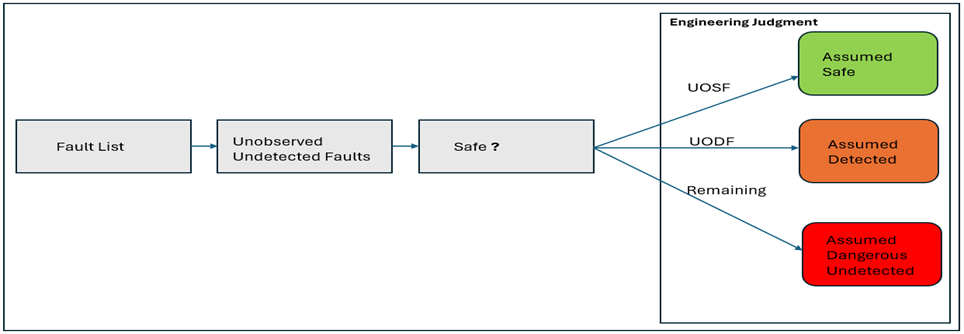
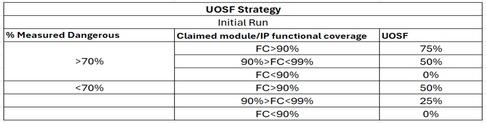
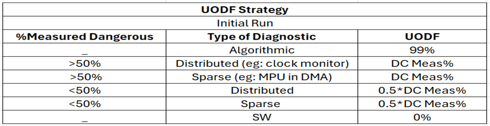
After applying all assumptions and barriers, if fault coverage remains insufficient, manual classification of faults with proper analysis and justification is necessary. Engineering Judgment (EJ) involves a set of rules (Unobserved Safeness Factor and Unobserved Detection Factor) for classifying unobserved faults as safe or detected. Justification is based on functional coverage (FC) and diagnostic coverage (DC).
Figure 6: Engineering Judgment
UOSF (Unobserved Safeness Factor) and UODF (Unobserved Detection Factor) are calculated based on:
Functional Coverage (FC): Indicates the effectiveness of workload for branch, toggle, or expression coverage. Higher FC implies well-simulated design, leading to a high UOSF (Unobserved Safeness Factor). Depending on the type of safety mechanism, high FC may also indicate that unobserved faults could potentially be detected (high UODF).
The calculation strategy for UOSF and UODF is as follows:
In summary, EJ involves evaluating unobserved faults using UOSF and UODF, with justification derived from functional and diagnostic coverage. Higher FC contributes to a higher UOSF and potentially a higher UODF, indicating the safety and detectability of unobserved faults by safety mechanisms.
Selection of window of opportunity
Transient analysis is used to examine faults that exist for a short period, known as transient faults. The time window during which faults are activated for propagation is termed the window of opportunity (WoO). Analysing the WoO for each node is critical yet complex, requiring a thorough review of waveforms and a deep understanding of data flow.
Sync events can aid in this process by serving as inputs to the Xcelium Fault Set Generator (XFSG) tool. By using clock signals as sync events, faults are injected immediately after the positive edge of the sync event signal. Identifying clocks in the design and utilizing them as sync events is essential since all flops in the design are activated based on different clock inputs. The XFSG tool takes a timing configuration file and waveform data (.shm file) as inputs to generate the fault list, considering the sync event timings.
For the initial fault injection (FI) run, starting time (after reset de assertion) and end time, along with the time interval between fault injections, can be specified. The fault generator injects the same fault in different time windows based on these parameters. Analysing the campaign output provides insights into which time windows activate or deactivate the most faults. This data aids in further analysis and minimizes the number of UU faults. Subsequent analysis focuses on identifying and understanding the WoO for the remaining UU faults.
Understanding tools limitation
The sync event flow only supports clock inputs; other signals cannot be used as sync events.
The serial fault engine considers all faults for the campaign, whereas it should normally only consider NS (Non-Simulatable) faults. This results in longer runtimes due to a higher number of fault simulations.
The FCM flow misbehaves when adding test cases supported by analog models, leading to fault hierarchy being skipped.
Summary and Future enhancement
Completing fault injection and achieving comprehensive diagnostic coverage on complex IPs within tight timelines presents considerable challenges. Our experiments and observations detailed above are aimed at overcoming these hurdles by optimizing runtimes and simplifying the analysis process.
The solutions discussed are not only applicable to the specific scenarios outlined but can be extrapolated to address similar challenges encountered with any IP. By implementing the strategies outlined, analysts can navigate through the complexities of fault injection and diagnostic coverage with greater ease and efficiency.
Looking ahead, there is potential for further enhancements in fault simulator tools. Developing a refined workflow that specifically targets UU faults for future campaigns, while excluding DD, DU, and safe faults, holds promise in reducing the overall fault set, streamlining runtimes, and facilitating more straightforward analysis processes.
Moreover, emphasizing the enhancement of FSV capabilities, especially in terms of visualizing stimulus to cover corner cases, is essential for ensuring a thorough fault analysis and achieving comprehensive diagnostic coverage across various IP designs.
In conclusion, by leveraging the insights and strategies discussed in this blog, the problem statement can be simplified, ultimately leading to more robust and reliable IP designs.
References
Fault Campaign Manager User Guide
Xcelium Fault Simulator User Guide
ISO 26262-1:2018 – Road vehicles — Functional safety
Felipe Augusto da Silva, Ahmet Cagri Bagbaba, Said Hamdioui, Christian Sauer, 2019, October, Efficient Methodology for ISO26262 Functional Safety Verification, 2019 IEEE 25th international symposiumoon On-Line testing and Robust system designing
That the contents of third-party articles/blogs published here on the website, and the interpretation of all information in the article/blogs such as data, maps, numbers, opinions etc. displayed in the article/blogs and views or the opinions expressed within the content are solely of the author's; and do not reflect the opinions and beliefs of NASSCOM or its affiliates in any manner. NASSCOM does not take any liability w.r.t. content in any manner and will not be liable in any manner whatsoever for any kind of liability arising out of any act, error or omission. The contents of third-party article/blogs published, are provided solely as convenience; and the presence of these articles/blogs should not, under any circumstances, be considered as an endorsement of the contents by NASSCOM in any manner; and if you chose to access these articles/blogs , you do so at your own risk.
In an era where digital experiences are becoming the norm, interacting with an AI chatbot no longer feels robotic. From retail support to mental health coaching, modern AI chatbots can carry on conversations that feel genuinely human. But how did we…
Q2 2025 saw USD 1.7 billion inflows, 29% rise compared to Q1 2025. Mumbai & Bengaluru together drove 39% of the investment inflows in H1 2025.
After a steady start in the first quarter, institutional investments in the Indian real…
The great travel reboot: Generative AI’s role in ending the planning chaos
Written by Sankar Subramaniam, Global Travel Industry Research Lead, Accenture
A few weeks ago, I tried to plan a short getaway. I opened my laptop and suddenly found…
In H12025, a leading product company announced plans to cut nearly 8,000 jobs as it ramped up AI-based automation efforts. Another big tech laid off its experienced IT position holder along with a significant amount of human capital. Read any recent…
India faces a mental health crisis that technology can help address. Recent studies indicate that approximately 15% of Indians experience mental health challenges, with youth aged 18-24 particularly vulnerable (Balamurugan et al., 2024). The…
The shift toward industry-focused technology
A quiet pressure has been seeping through boardrooms and C-suite conversations: technology stacks are being refactored so that sectors, rather than vendors, dictate first principles. Instead of debating…